The circle map

is a fundamental model describing many dissipative nonlinear systems like a self-oscillator under external periodic driving, Josephson junction in a microwave field, space charge density waves in solid-state physics, a pendulum with periodic external force. In studies concerning medical and biological problems, the circle map appears as a model of cardiac rhythms.

The circle map is not only a qualitative model, but a representative of a class of quantitative universality associated with a transition to chaos via quasiperiodic motion. The most well studied case relates to the ratio of basic frequencies, or the rotation number, equal to the golden mean constant w=(5^1/2-1)/2. It corresponds to the GM critical point at K=1 and r=r_c=0.60666106347011... It was reported on many experiments, in which the universal regularities associated with the GM critical point were observed and documented, e.g. in fluid convection and in in electronic oscillators in presence of external driving.

In real physical systems, effect of noise takes place inevitably. Let us turn to a circle map with added random force:

where x_n is a sequence of statistically independent random numbers with a zero mean and fixed variance s, e is a parameter of intensity of noise supposed to be small.

Below we show charts of the Lyapunov exponent for the circle map on the parameter plane (r, K) without noise (the first diagram, where location of the GM point is marked) and in presence of noise (the second and the third diagram). For each pixel corresponding to certain r and K, we compute the Lyapunov exponent and code the pixel with colors from dark to light for values from minus infinity to zero, and black for positive values. The domains of periodic dynamics in the system without noise are called the Arnold tongues. They are gray colored formations in a form of acute edges, inside which the rotation number values are rational. Between them the quasiperiodic regimes occur with irrational rotation numbers.

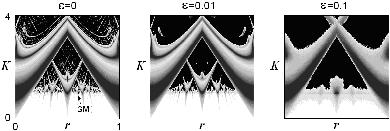
In presence of noise, the periodic or quasiperiodic dynamics does not occur in exact sense, but the picture of characteristic domains on the Lyapunov chart remains visible, at least for small and moderate noise intensities. We can speak either on "noisy periodic regime", when the Lyapunov exponent is notably negative, on "noisy quasiperiodic", if it is close to zero, or of "noisy chaotic" as the Lyapunov exponent is positive. The Lyapunov charts allow to distinguish visually these regimes. In a sense, the effect of noise looks rather trivial: the subtle details of the picture appear to be smeared off.

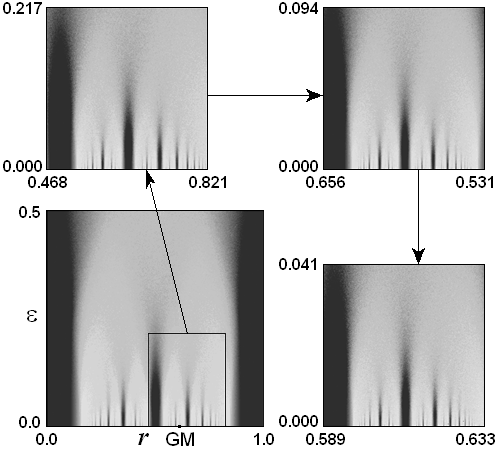
The following figure shows phase portraits of the attractors on the iteration diagrams, plots of x_n+Fk versus x_n, where F_k is one of the Fibonacci numbers. The diagrams are presented for F₆ = 8 at the parameter values K and r associated with the critical point GM.

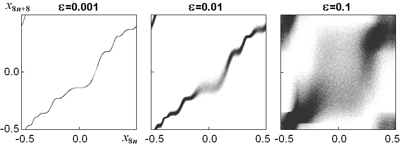
The first picture corresponds to a very weak noise, the second and the third to larger intesities (see indicated values of e). Observe successive smearing of subtle and than more large scale structural details of the attractor as the noise intensity grows.

As known, without noise near the critical point GM definite scaling regularities take place [Shenker, Ostlund, Rand, Feigenbaum, Kadanoff], hence, one can think that effect of noise also must be associated with some properties of universality and scaling. The renormalization group (RG) analysis suggested by Hamm and Graham [Hamm and Graham, 1992] leads to a conclusion of existence of a universal constant, which indicates how much the noise intensity has to be decreased to observe each next level of the small-scale structure in a vicinity of the GM critical point: g=2.3061852653. (The content of the RG analysis is here.)

More general formulation of the scaling property is the following.

Let us suppose that with deflection of r from the value corresponding to the golden-mean rotation number Dr and K close to K_c=1 in presence of noise e a certain regime of behavior takes place. Then, at Dr decreased by factor d1=2.83361066, DK decreased by factor d2=1.66042438, and the noise intensity e/g the statistically similar regime will occur with the larger by factor W=1/w=(5^1/2+1)/2 characteristic time scale. The probability distribution for the variable x near the inflection point will be similar to the original with characteristic scale in x decreased by the factor a=-1.28857455. In a region of small deflections from the criticality, and of small noise intensities, the distribution law, as believed, is universal, i.e. does not depend on details of the distribution and of correlation properties of the initial noise (with sufficiently fast damping of the tails of the correlation function).

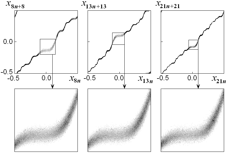
Let us consider some computer illustrations of the mentioned scaling. We start with a series of plots, each of which depicts a noisy attractor on the iteration diagrams in coordinates x(nF_k), x((n+1)F_k, where F_k is a Fibonacci number with k=6, 7, 8. From one picture to another the noise parameter is decreased by factor g. Values of K and r correspond to the critical point GM. On each plot we select a fragment near the origin shown separately with magnification. Similarity of the objects observed on these magnified pictures illustrates the expected scaling property in the system with noise.

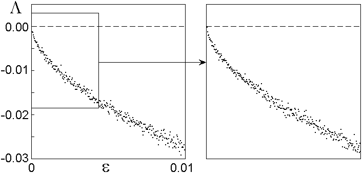
Let us turn now to diagrams shown the rotation number

dependence on the parameter r at K=1. The basic plot and the first inset relate to the circle map with noise at e=0.1. The other pictures show fragments with growing magnification along the horizontal and vertical axes, respectively, with factors d₁ and W², and decreasing noise intensity by factor g. Observe obvious similarity of the plots on the smaller diagrams.

The next diagram depicts a dependence of the Lyapunov exponent on the noise intensity at K and r corresponding to the GM critical point. As seen, presence of noise leads to decrease of the Lyapunov exponent, i.e. facilitates stabilization (in contrast to the situation of the Feigenbaum transition, for which the noise gives rise no increase of the Lyapunov exponent). In the inset a fragment of the plot is shown with rescaling along horizontal by factor g and along vertical by factor W=(5^1/2-1)/2. Similarity of both pictures illustrates the expected scaling property.

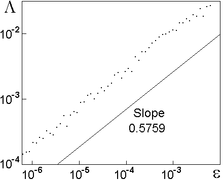
One more way to demonstrate scaling consists in plotting of the Lyapunov exponent versus the noise intensity in the double logarithmic scale. Observe that the dots are located in average along a straight line with the slope coefficient log_gW=0.5759, where W=(5^1/2+1)/2.

Another series of illustrations contains the Lyapunov charts relating to the critical value of the parameter K=1. The horizontal axis is that of parameter r, and the vertical one of the noise intensity parameter e. The gray tones from dark to light code Lyapunov exponent values from minus infinity to zero, and black corresponds to positive values. For each next picture for illustration of the scaling property the horizontal and vertical scales are changed by a factor, respectively, d₁ and g. Additionally, a rule of color coding is redefined to take into account the characteristic time scale by the factor W=(5^1/2+1)/2.

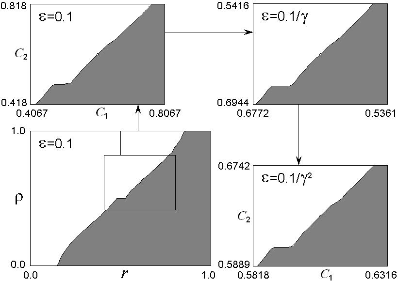
Finally, the last series of diagrams represents the Lyapunov charts illustrating the scaling property of the picture of the Arnold tongues. For this, it is necessary to introduce certain special local coordinates (C₁,C₂) on the parameter plane near the GM critical point: One coordinate axis is directed along the critical line K=1, and the second one along the curve of constant rotation number defined in absence of the noise.

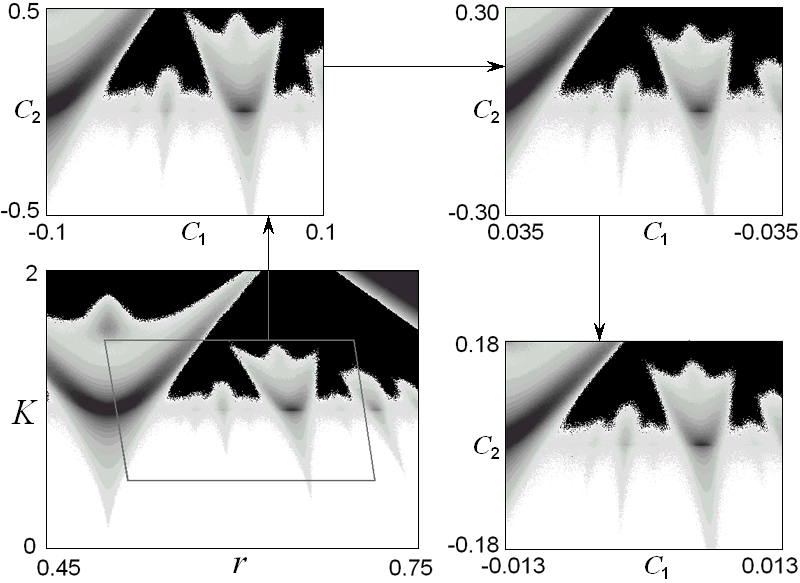
The main diagram is a Lyapunov chart on the plane (r,K) at the noise intensity e=0.03. The first inset shows an interior of the selected parallelogram in the local coordinates, which are expressed wia the parameters of the circle map as follows

The other two pictures are obtained with the noise intensity parameter decreased, respectively, by g and g² times. The horizontal and vertical scales correspond to magnification from one picture to another by factors d₁ and d₂, with respective redefinition of the color coding rule for the Lyapunov exponent.

• Effect of noise on the Feigenbaum transition
• Effect of noise on the golden-mean quasiperiodicity at the chaos threshold
• Effect of noise on the period-tripling
• Effect of noise on the torus doubling terminal criticality