Properties and quantitative characteristics of strange nonchaotic attractors

Lyapunov exponents

For quasiperiodically driven one-dimensional maps, there is one non-trivial Lyapunov exponent L. For SNA, as well as for a torus, it is negative. However, the attractor consists of a set of orbits, hence, a presence of individual unstable trajectories, which have L>0, cannot be excluded. (A set of such orbits should be thin, of zero measure, so that the Lyapunov exponent averaged over the entire attractor should be negative.) For example, in the model x_n+1=l th x_ncos 2pq_n, q_n+1=q_n+w (mod 1), at l>1, a set of points on the axis x=0 with phases q_n=1/4+nw forms just such an exclusive trajectory. This is just the property, which is a distinctive feature of SNA in comparison with the torus-attractor. In numerical computations, presence of the unstable orbits on the attractor may be detected from statistics of local, or finite-time Lyapunov exponents.

For a one-dimensional quasiperiodically forced map x_n+1=f(x_n, q_n), q_n+1=q_n+w (mod 1), let us define a value

where a dash designates derivative over the first argument, and an initial point (x₀, q₀) belongs to the attractor. Performing the computation many times, we get a set of values L_N, for which we can introduce a distribution function F(L).

Let us consider as an example the driven quadratic map x_n+1=l - x_n²+ecos 2pq_n, q_n+1=q_n+w (mod 1).

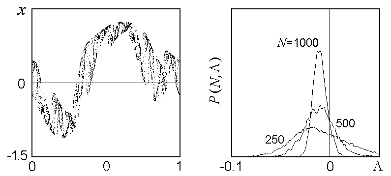
In the following figure to the left we show a portrait of SNA at l=0.8, e=0.45 with the estimated value of the Lyapunov exponent L=-0.010. The right diagram shows the distribution functions obtained numerically L_N at N=250, 500 and 1000. They have a form of a one-hump curve, and location of the maximum just corresponds to the Lyapunov exponent L. With grows of N, a width of the distribution decreases, but it keeps a 'tail' in positive L_N. It indicates presence of locally unstable orbits on the attractor. A fraction of events of generation of positive local exponents L_N decreases, but never vanishes although tends to zero limit for infinitely large N.

Phase sensitivity exponent

Let us consider a possibility to reveal quantitatively a non-smooth dependence of the coordinate variable on the phase intrinsic to SNA. For this, it is natural to trace evolution in a course of iterations for the value . Scheme of the computation consists in simultaneous iterations of the original map together with the relation obtained as a derivative in respect to the phase:

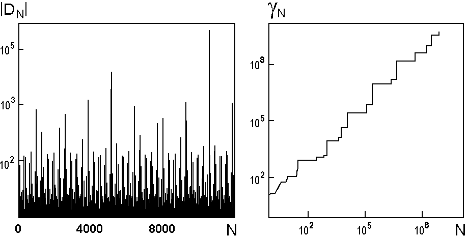
In the following figure, the left diagram shows a plot of D_N versus a number of iterations in the model with f(x, q)=l th xcos 2pq in the case of SNA, at l=1.5, w=(5^1/2-1)/2. It looks like a set of peaks, and the height of the maximal peak registered over N iterations grows with N. The right diagram is a plot of this maximum versus N in double logarithmic scale. Observe, that the growth follows, in average, to a power law (the power index depends, in general, on the examined orbit.)

To obtain a characteristic relating to the entire attractor, Pikovsky and Feudel (Chaos, 5, 1995, 253) suggested determining the phase sensitivity exponent as a maximal value of the power index over all orbits on the attractor:

For the present example, m=0,97. On the other hand, for a torus-attractor, obviously, m=0. Thus, in principle, the phase sensitivity exponent is a tool to distinguish SNA and torus.

Fractal structure and dimension of SNA

Although qualification of SNA as a 'geometrically strange object' is one of the main points in its definition, the question on fractal properties of SNA is studied not so well. In accordance to M.Ding et al. (Phys. Lett., 1989, A137, 167), SNAs in the pitchfork bifurcation model and in the driven circle map has fractal dimension (capacity)

and information dimension

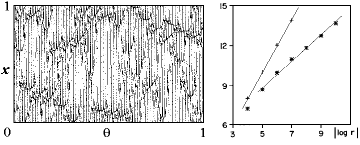
Here N is a number of elements for covering by boxes of size e, p_i is a probability of presense in the i-th box. As an example, the following figure shows in the left diagram a portrait of SNA in the driven circle map at K=0.95, e=1.2, r=0.2841, and the right diagram is the double logarithmic plot used for the estimate of the dimensions. Crosses relate to the estimate of the capacity D₀, and stars to the information dimension D₁, which are determined by a slope of the approximating straight lines.

Spectral properties of SNA

Fourier analysis is a commonly used method of signal processing in studies of dynamics, in particular, in experiments. Discussing possible types of spectra, let us take the following way of reasoning. As we have some sequence x_n to be analyzed, let us construct an 'accumulating sum' S(W,N)=Sx_neⁱWn, where W is a parameter, and examine a dependence of the complex value S(W,N) on the number of terms in the sum N. For periodic and quasiperiodic sequences on some discrete set of values W we get S(W,N)~N, i.e. |S(W,N)|²~N², else |S(W,N)|²-->0. This is a discrete spectrum. For random or chaotic sequences the evolution of S looks like a random walk (diffusion) on the complex plane, and in this case S(W,N)~N^1/2, and |S(W,N)|²~N. This is a continuous spectrum, such spectra are considered in the theory of stationary random processes (the Wiener-Khinchin theory). For sequences generated by SNA the walk of the value of S(W,N) on the complex plane is of fractal nature, forming structures with nontrivial properties of scaling. Asymptotic behavior under increase of N obeys a relation |S(W,N)|²~N^b, where the index b is between 1 and 2 and depends on W. This case is referred to as a singular-continuous spectrum. In the following figure the right diagram shows three samples of random walk corresponding to the continuous spectrum, and the right one illustrates for comparison the fractal walk of the spectral sums for the case of SNA (the hyperbolic tangent map, l=1.5). The numbers indicate values of the normalized frequency parameter W/2p.

Rational approximations and nature of SNA

Any irrational number from interval (0,1) can be represented as a continued fraction

where a_i are positive integers. The rational approximant of order k corresponds to the sequence of elements cut at the k-th position:

Then, lim r_k=r, and the terms of the rational sequence r_k appear as the best approximants of the irrational. For the 'golden mean' we have w=(5^1/2-1)/2=<1,1,1,...>, and the rational approximants are given by ratios of the Fibonacci numbers: F_k/F_k+1, где F₀=0, F₁=1, F_k+1=F_k+F_k-1.

If we take a rational approximant of order k instead of the irrational frequency in a model of forced map

then, the external driving will be periodic, of period q_k. In contrast to the the quasiperiodic case, when the phase variable in ergodic manner visits a dense set on the unit interval, now the set is finite: (q₀, q₁,...q_qk-1). In dependence on q₀ we will observe, in general, different regimes and attractors. Therefore, the initial phase q₀ plays a role of an additional parameter. As we intend on a basis of examination of the rational approximations to draw conclusions about behavior in the quasiperiodic case, we should account all situations, which occur at arbitrary initial phases q₀ in an interval from 0 to 1/q_k.

The following figure shows charts of dynamical regimes on the parameter plane of the forced quadratic map at rational approximations (a-c) and at irrational frequency w=(5^1/2-1)/2 (г). A comparison of the charts shows that the areas of regular quasiperiodic dynamics in the diagram (d) (tori T1, T2, T4) are associated with areas of periodic regimes (cycles) in the diagrams (a-c). In domain, where SNA appears in the quasiperiodic case, the charts for rational approximations manifest 'flicker' of regimes of different kind, in subtle dependence on the initial phase and order of the approximation.

Pikovsky and Feudel (Chaos, 5, 1995, 253) suggested a hypothesis for a necessary condition of existence of SNA. Namely, at a rational approximation of the frequency parameter, the system demonstrates bifurcations in dependence on the initial phase, and this property persists under increase of the order of the approximation. Qualitatively, in terms of the systems obtained from the rational approximations, one can imagine somewhat like a slow drift of the phase parameter accompanied with permanent bifurcations in a course of state evolution in the system. This may be regarded as a mechanism of appearance of SNA.