|
Mandelbrot and Julia sets |
One special chapter of nonlinear dynamics elaborated deeply by mathematicians consists in a study of iterated maps defined by analytic functions of complex variable. A classic object is the complex quadratic map
![]()
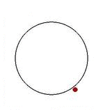
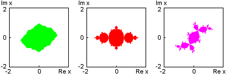
At с=0 the behavior is rather obvious: for |z0|>1 the result of iterations will tend to infinity, and for |z0|<1 one observes residence in a bounded part of the complex plane. The boundary between these two kinds of behavior is a unit circle |z0|=1. At other values of the complex parameter c a set on the complex plane z, separating the analogous two types of behavior is rather complicated and nontrivial (fractal). It is called a Julia set (see examples in the picture).
 On the other hand, if we fix initial condition
z0=0 and consider behavior in dependence on the
complex parameter c,
then, at some values the iterations will escape to infinity, and
at other will stay in a bounded domain.
A set of points associated with this last situation
on the complex plane
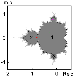
c is called the Mandelbrot set (see picture to the right). Figures 1, 2, 3
designate periods of dynamics observed at several basic leaves of the "cactus".
The color dots mark parameter values at which the Julia sets have been plotted in the previous
figure.
On the other hand, if we fix initial condition
z0=0 and consider behavior in dependence on the
complex parameter c,
then, at some values the iterations will escape to infinity, and
at other will stay in a bounded domain.
A set of points associated with this last situation
on the complex plane
c is called the Mandelbrot set (see picture to the right). Figures 1, 2, 3
designate periods of dynamics observed at several basic leaves of the "cactus".
The color dots mark parameter values at which the Julia sets have been plotted in the previous
figure.
Remark. There is also a separate segment of our site specially devoted to complex maps.
The idea of physical realization of phenomena of complex dynamics
we suggest here is based on the method of complex amplitudes
well known in the oscillation and wave theory.
Let us have an oscillatory process on a frequency
w0 with slow complex amplitude
a(t):
Let us consider a system of two coupled non-autonomous oscillators
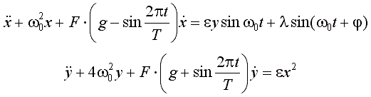
The first oscillator has a characteristic frequency w0,
and the second one has a frequency twice larger.
Parameters controlling dissipation in the both oscillators
slowly swing in counter-phase with period T, which equals an integer number
of periods of basic oscillations.
Parameter g is supposed to be positive, less than 1. Thus,
been in average positive, on a certain part of swing period the dissipation
becomes negative. On this interval the oscillator is active (the oscillations grow).
On the rest part of the swing period it is passive (the oscillations decay).
 Let us assume that at the moment of beginning of the active stage of the
second oscillator, the first one oscillates with complex amplitude a:
x(t)~Re[a(t)exp(iw0t)].
The resonance priming for the second oscillator is the second harmonic
component produced by the nonlinear quadratic transformation of te signal from the first
oscillator,
Re[a2exp(2iw0t)].
As follows, the complex amplitude of the second oscillator on its active stage
will be proportional to
a2. Mixing with auxiliary signal
(see the right-hand side of the first equation) yields a difference frequency
component w0 with amplitude proportional to
a2. Then, a sum of it with an additional oscillatory term of frequency
w0, amplitude
l and phase j
produces a priming for the complex amplitude of the first oscillator of form a2
plus a complex constant.
Hence, the stroboscopic map for the complex amplitude
will correspond, at least in a definite approximation,
to the complex quadratic map.
The role of complex parameter plays the complex number with modulus
l and argument
j. In dependence on this parameter, it
may happen that the solution for the equations of coupled non-autonomous
oscillators remains bounded for initial conditions from
some domain of the phase space, or escapes to infinity.
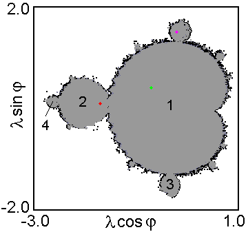
On the parameter plane diagram shown to the right the gray color
corresponds to bounded dynamics observed in computations, and white
to the escape. The computations were performed for
w0=2p,
T=10, F=7, g=0.5, e=1.
The object manifests an obvious similarity with the Mandelbrot set
for the complex quadratic map.
The figures 1, 2, 3 designate the leaves, where dynamics of periods
T, 2T, 3T take place, respectively.
Let us assume that at the moment of beginning of the active stage of the
second oscillator, the first one oscillates with complex amplitude a:
x(t)~Re[a(t)exp(iw0t)].
The resonance priming for the second oscillator is the second harmonic
component produced by the nonlinear quadratic transformation of te signal from the first
oscillator,
Re[a2exp(2iw0t)].
As follows, the complex amplitude of the second oscillator on its active stage
will be proportional to
a2. Mixing with auxiliary signal
(see the right-hand side of the first equation) yields a difference frequency
component w0 with amplitude proportional to
a2. Then, a sum of it with an additional oscillatory term of frequency
w0, amplitude
l and phase j
produces a priming for the complex amplitude of the first oscillator of form a2
plus a complex constant.
Hence, the stroboscopic map for the complex amplitude
will correspond, at least in a definite approximation,
to the complex quadratic map.
The role of complex parameter plays the complex number with modulus
l and argument
j. In dependence on this parameter, it
may happen that the solution for the equations of coupled non-autonomous
oscillators remains bounded for initial conditions from
some domain of the phase space, or escapes to infinity.
On the parameter plane diagram shown to the right the gray color
corresponds to bounded dynamics observed in computations, and white
to the escape. The computations were performed for
w0=2p,
T=10, F=7, g=0.5, e=1.
The object manifests an obvious similarity with the Mandelbrot set
for the complex quadratic map.
The figures 1, 2, 3 designate the leaves, where dynamics of periods
T, 2T, 3T take place, respectively.
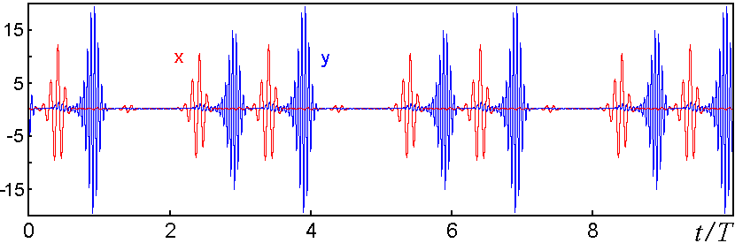
The next picture illustrates oscillations observed in one of the regimes in the leaf 3. We present time dependences for variables x and y, which correspond to two subsystems.
Obviously, a type of regime is determined by the priming signal, which acts in the initial part of the active stage and is formed as a composition of the signal from the partner oscillator and that of the external force. Essential are the phase relations of these two signals, which determine subtle structure of leaves of the "cactus" in the parameter plane.
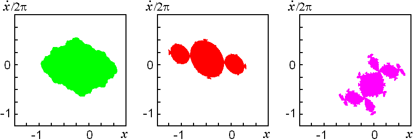
For points marked on the "cactus" diagram in colors we plot diagrams on phase plane of the first oscillator (x, dx/dt) in stroboscopic section. They represent basins of attractors located in a bounded domain. They may be compared with portraits of Julia sets of the complex quadratic map in the first diagram on this page.
The data we have presented here demonstrate conclusively many features intrinsic to dynamics of iterative complex analytic maps. Indeed, we reproduce in particular such objects as sets of Julia and Mandelbrot, at least up to notable details. The question either the correspondence takes place as well on arbitrarily fine scales of fractal structures remains open yet and, for sure, deserves further studies.