For realization of hyperbolic chaos by manipulating phases of oscillations during transfer of the excitation between the alternately active oscillators, very appropriate is a class of parametric systems well known in the oscillator theory and applications. Such systems may be designed on a different physical base, e.g. in electronics, mechanics, nonlinear optics.

One commonly used scheme of a parametric generator consists of two partial oscillators coupled via a reactive (non-dissipative) element with a time-dependent parameter. If the frequencies of the oscillators w₁, w₂, and the frequency of the parameter variation (pump frequency) w₃ obey a condition of the parametric resonance w₃=w₁+w₂, then, in the partial oscillators simultaneous excitation of the oscillations occurs. Saturation of the amplitudes may be reached with introduction of nonlinear dissipation.

Let us turn to a system composed of two such subsystems, A and B (see the figure). The frequencies are selected in such way that w₂=2w₁ and w₃=3w₁. (The condition of the parametric resonance is valid, obviously.) In each subsystem, an oscillator of frequency w₁ is supposed to be linked via a quadratic nonlinear element with an oscillator of frequency w₂, relating to the partner subsystem. Because of the accepted frequency ratio, the effect of one oscillator onto another will be resonance (strong).

Let us assume now that the pump is applied alternately to one and another subsystem. Then, the operation of the device consists of alternating parametric excitation of two subsystems A and B and decay of the oscillations in the intermediate time intervals.

The model is governed by the equations

Here x_1,2 and y_1,2 are generalized coordinates of two pairs of the oscillators of frequencies w₁ and w₂=2 w₁. Parameter k designates the intensity of pump at the frequency w₃=3w₁. Parameter e is responsible for the nonlinear coupling between the oscillators relating to different subsystems. The functions f and g define a slow periodic variation of the pump amplitude, in such way that for two subsystems it oscillates in counter-phase:

The modulation period is assumed to contain an integer number of periods of the basic pump frequency, i.e. T=2pN/w₃, with N integer.

At N>>1 one can use the slow-amplitude method. Let us set

where A and B are complex variables slowly varying in time. After substitution in the equation, multiplication by the exponent, and averaging over a period of fast oscillations, with account of the accepted frequency ratio for w_1,2,3, we obtain:

With e=0, the system decomposes to two isolated subsystems, A and B.

Let us consider one of them, say, A. Without dissipation and at constant amplitude of the pump, it is governed by the amplitude equations

At large time, the solution behaves as

where R and Ф are constants determined by the initial conditions. It corresponds to

Thus, the first and the second harmonic components of the oscillations developing due to the parametric instability possess the phase shift determining by one and the same constant Ф depending on the initial conditions. With taking into account the nonlinear dissipation, the amplitude will saturate, but the noted phase condition persists.

Let us turn now to the situation of alternating pump in the subsystems in presence of nonzero coupling. The excitation of a subsystem A or B under the effect of the pump will occur in presence of a weak driving from the partner subsystem upon the partial oscillator of frequency w₂=2w₁. It is produced by the second harmonic component transformed from the oscillator of frequency w₁. This second harmonic component has doubled phase, which is inherited by the stimulated oscillator. On a complete period of pump modulation, the transformation of phase will be determined approximately by the map Ф_new=4Ф_old+const (mod 2p), which relates to the family of Bernoulli maps. Its dynamics is chaotic with the Lyapunov exponent L=ln 4=1.386.

For accurate description of the dynamics in discrete time, an instantaneous state of the system at t=t_n has to be assigned by means of an 8-dimensional vector X_n. Solving the equations on a time interval T with initial conditions X_n we obtain a set of variables determining the new state X_n+1. Introducing the function mapping the 8-dimensional space into itself, we arrive at the Poincare map: X_n+1=T(X_n). (In accordance with known results of the differential equation theory, this map is one-to-one and differentiable.) For definition of the phase variable Ф we may use an oscillator of frequency w₁ relating to the subsystem active at t_n. With one iteration of the Poincare map, in the 8-dimensional phase space we will have 4-fold expansion along the direction associated with the phase and strong compression along other dimensions. As we assert, the Poincare map has, in fact, a uniformly hyperbolic attractor relating to the family of the Smale - Williams solenoids.

Let us turn to numerical simulation of the dynamics. It is convenient to set w₁=2p, w₂=4p, w₃=6p, that corresponds to unit period of oscillations in the first oscillators of the both subsystems. Below, in the figure we show typical time records corresponding to a sustained regime of parametric oscillations for the variables x and y on one period of the pump modulation T=40 at e=0.5, k=35, a=0.6, b=0.01.

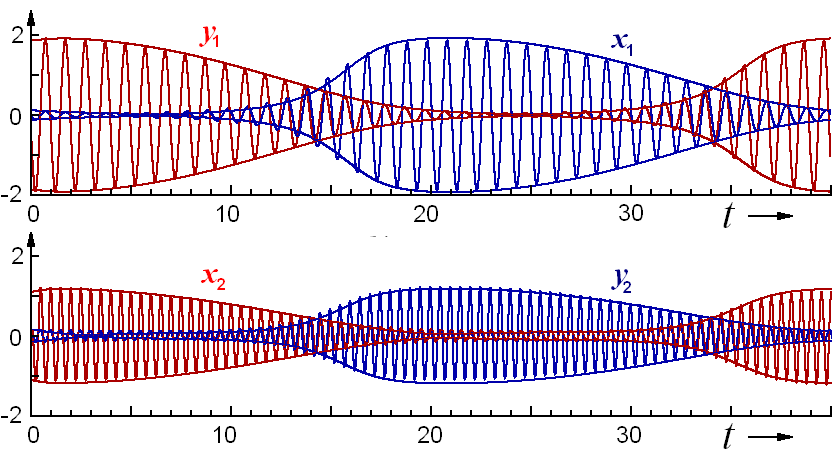
The red curves relate to the subsystem A, and blue to the subsystem B. Observe that both subsystems become active turn by turn, in accordance with application of the pump. Each subsystem generates output sequence of pulses with high-frequency carrier, following with the period of the pump modulation. Nevertheless, the signal is non-periodic: the phase of the high-frequency oscillations varies chaotically from one pulse to another. In the figure we present as well the amplitude curves obtained from the numerical solution of the shortened equations. Because of evident good agreement we restrict further consideration with discussion of the dynamics described by the amplitude equations.

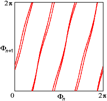The diagram to the right is an iteration plot for phases corresponding to successive stages of excitation of one subsystem. Along the horizontal axis a phase in the subsystem B is plotted relating to an instant t_n=nT, and along the vertical to the moment t_n+1. The diagram is obtained from the numerical solution of the amplitude equations. The phase is determined as Ф_n=argB(t_n). (We emphasize that the definition relates to the stage of activity of the subsystem, when the amplitude is surely far from zero.) As seen from the diagram, a single turn around the circle for pre-image Ф_n gives rise to a four-fold turn for the image Ф_n+1. It implies that the map for the phases relates to the same topological type as the Bernoulli map Ф_new=4Ф_old+const. (Weak splitting of the branches is apparently insignificant.)

A complete spectrum of Lyapunov exponents for the attractor of the Poincare map at the above parameters in accordance with the computations is the following:

Note that the largest exponent agrees well with the value ln 4 corresponding to the approximate description with the Bernoulli map. Others are negative that implies strong compression of the phase volume element along the respective dimensions in the phase space. An estimate of the dimension of the attractor by Kaplan - Yorke formula yields D=1.26 for the attractor of the Poincare map. Respectively, for the attractor of the original system, which is embedded in the 9-dimensional extended phase space, the dimension is 2.26.

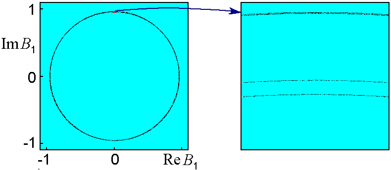
The picture below shows phase portrait of the attractor in the Poincare cross- section, in projection onto the plane of variables of the first oscillator of the second subsystem. A panel to the right shows a magnified fragment, where one can see some details of the subtle transversal fractal structure of the attractor.

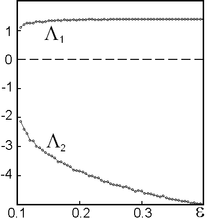The last plot shows two largest Lyapunov exponents versus the parameter of coupling between the subsystems at fixed other parameters. In the whole range one exponent is positive, and others are negative. The dependence of the largest exponent on the parameters appears to be smooth, without abrupt drops. Observe that in a wide parameter range the value of the largest exponent remains close to ln 4.

The scheme of the parametric generator of chaos we consider opens a possibility of realization of chaotic regimes insensitive to variation of parameters and to details of construction in systems of different physical nature.